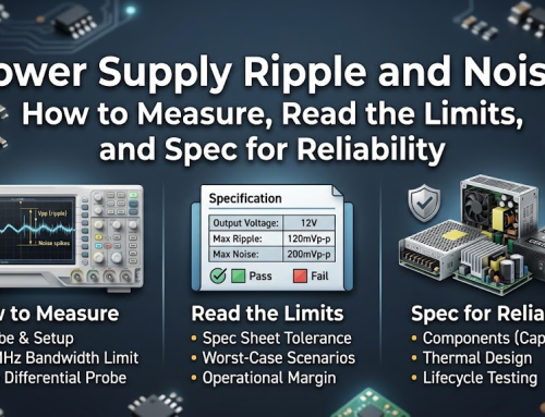
How to Measure Power Supply Ripple and Noise: One Wrong Probe Connection Turns a Good Supply Into a Failed One
The datasheet says output ripple ≤150 mVpp. A customer hooks up a brand-new 100 MHz scope to the output, uses the alligator clip lead that came in the probe kit, reads 250 mVpp, and sends an email explaining that we’re 67% over spec.
We got the same supply back on the bench and measured it properly: 42 mVpp.
The supply hadn’t changed. The probe connection had. This happens somewhere in the industry every week, and most of the time the power supply is innocent.
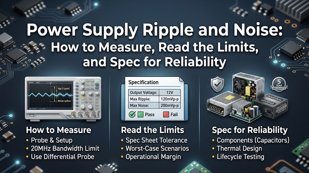
This article covers what output ripple and noise (PARD — Periodic And Random Disturbance) actually means, where the 20 MHz bandwidth limit comes from, why the ground lead in your probe kit has to come off, why light-load ripple is often worse than full load, and the five measurement traps that get good supplies rejected.
First, what you’re measuring
PARD is everything non-DC sitting on top of the DC output. It splits into two halves with completely different origins.
Periodic — the part that repeats:
- Mains rectification ripple at twice the line frequency: 100 Hz on a 50 Hz grid, 120 Hz on 60 Hz. It comes from the bulk capacitor discharging between mains peaks
- Switching-frequency ripple, typically 50 kHz–500 kHz, plus its harmonics
Random disturbance — the part that doesn’t:
- MOSFET turn-off ringing on the switch node (Vds), coupled through the transformer to the output as MHz-range spikes
- Output rectifier reverse recovery (trr), which produces a sharp current step and a matching voltage spike
- Transformer leakage inductance ringing tens of MHz
PARD is almost always quoted peak-to-peak in mVpp, because what upsets a sensitive load is the spike amplitude, not the RMS average. If you’re putting this into a custom spec, it belongs at item 5 of the custom power supply quotation checklist — naming the bandwidth limit alongside the mVpp figure, or the number is unverifiable.
One boundary that has to be clear: PARD is not load regulation, and it is not transient response.
| Metric | What it measures | Stimulus | Unit |
| PARD (ripple and noise) | AC content on the DC output at steady state | Nothing — load and input stable | mVpp |
| Line regulation | DC output shift from input change | Input sweep (e.g. 90→264 VAC) | % or mV |
| Load regulation | DC output shift from load change | Static load step (e.g. 10%→100%) | % or mV |
| Transient response | Dip and recovery from a load step | Dynamic step at defined dI/dt | mV dip / µs |
A supply can have excellent regulation and poor PARD, or the reverse. When a datasheet gives you a single “ripple” line, confirm which of the four it is.
The 20 MHz limit isn’t hiding noise — it’s stopping you from measuring your own probe
Every credible ripple specification is produced with the scope’s 20 MHz bandwidth limit enabled. That isn’t industry habit, it’s written into standards:
- JEITA RC-9131C (Japan Electronics and Information Technology Industries Association)
- Intel ATX12V / ATX12VO power supply design guide
- SSI server power supply specification
All three specify a 20 MHz bandwidth limit and define the termination method.
The reason is straightforward. Above roughly 20 MHz, the loop formed by the probe tip and its ground return is effectively a small antenna, and the probe and scope front end ring on their own. Open the bandwidth to 100 MHz or 1 GHz and you’re mostly measuring the measurement system, not the supply.
The 20 MHz window is chosen deliberately. It covers everything a downstream load actually responds to — bulk capacitor ripple, switching ripple, and the leading edge of switching spikes — while excluding radiated hash that no load-side decoupling network would ever pass. Spike leading edges still show up. Radiated overshoot doesn’t.
Measuring with the bandwidth wide open is the number one cause of false failures.
How you connect the probe matters more than what the probe cost
This is the section worth reading twice.
The 6-inch (≈150 mm) alligator ground lead that ships with a standard 10× passive probe carries roughly 150–250 nH of inductance. That inductance resonates with the probe and scope input capacitance, and manufactures spikes that don’t exist at the output.
One set of measurements makes the point. Same 12 V buck output, 2 A full load, only the grounding changed:
| Grounding | Bandwidth | Scope reading | Estimated true value |
| Alligator clip to distant GND | 20 MHz | 180 mVpp | ≈40 mVpp |
| Alligator clip to near GND | 20 MHz | 95 mVpp | ≈35 mVpp |
| Spring ground | Full bandwidth | 68 mVpp | ≈32 mVpp |
| Spring ground | 20 MHz limit | 42 mVpp | 42 mVpp |
Same supply. 180 mV or 42 mV — a factor of 4.3.
What decides the result is the ground loop, not how expensive the probe is.
The correct setup:
- Remove the alligator lead. Fit the probe’s spring ground accessory. No spring to hand? Bend one from stiff copper wire, keeping it under 10 mm
- Tip on the output capacitor’s positive terminal, spring on that same capacitor’s negative terminal. Keep the loop area under about 1 square inch (≈6.5 cm²)
- Probe at the final output filter capacitor. Not beside the inductor, not arbitrarily at an IC pin
- Switch to AC coupling. 50 mVpp on a 12 V rail is a tiny AC signal on top of a large DC pedestal. Leave it on DC coupling and the DC level eats the vertical range, flattening the ripple detail
- Tack a small MLCC (say 1 µF) at the probe tip to emulate the local decoupling a real load presents. Measure with and without — the difference tells you what’s real and what’s probe artefact
- Probe attenuation: 10× with a spring ground is the daily default. For very small ripple (<20 mVpp), 1× has lower noise, but 1× probes typically only reach 6–10 MHz bandwidth and will roll off the high-frequency content themselves. Readings won’t match between the two; that’s normal — just record which you used
If the board has no ground plane, or the test point is far from the scope, use a differential probe or an SMA cable with 50 Ω termination (SMA shield soldered directly to the output capacitor’s GND pad). A differential probe floats both inputs and rejects common-mode far better; entry-level units start in the low hundreds of dollars.
Three findings that run against intuition
1. Light load often produces more ripple than full load
The default assumption is that ripple grows with load. Full load does produce the largest continuous switching ripple current, but light load is a different regime.
Many converters drop into discontinuous conduction mode (DCM), pulse skipping or burst mode at light load. They deliver energy in irregular packets, and the ripple is larger and more irregular than at nominal load under smooth continuous conduction.
That’s exactly why standards fix the load condition, and why you have to measure 10% load, not just 50%. The light-load reading is frequently the worst one on the sheet.
Cover four points as a matter of routine: 10%, 50%, 100%, plus a 50%→100% dynamic step (that’s transient response, a separate metric).
2. Ripple is worse at low input voltage, not high
Input voltage affects ripple, and the direction is backwards from what most people expect.
At 90 VAC input the bulk capacitor discharges deeper between mains peaks than it does at 264 VAC, so the 100/120 Hz twice-line component is significantly larger.
Measuring only at 50% load and 230 VAC produces a flattering number that hides both worst cases: light-load DCM and low-line input. A proper matrix covers 90 VAC and 264 VAC across three load points.
3. Grounding the probe to the chassis inflates the reading
Ripple is a differential quantity — the potential difference between the two output terminals (V+ to V−). That’s what the load actually sees.
But there’s also common-mode noise on the output: the shared potential of both terminals relative to earth or chassis, driven by the transformer’s primary-to-secondary coupling capacitance. If you reference the probe ground to the chassis while the output is floating, common-mode noise gets added straight into the reading.
So: measure differentially across the load (V+ to V−), never output-to-chassis. Output common-mode is normally clamped with a small output Y capacitor (around 1 nF) — a separate design path from differential filtering.
Typical targets by application
“How much ripple is acceptable” is meaningless without the application. Tighter costs more, every time.
| Application | Rail | Typical target (mVpp @ 20 MHz) | Notes |
| ATX 12 V | +12 V | ≤120 | Intel ATX12V design guide |
| ATX logic rails | +3.3 V / +5 V | ≤50 | |
| USB-PD adapter | 5–48 V | ≤100 | PPS modes can be tighter |
| Industrial 24 V / 48 V | +24 V / +48 V | ≈1% of Vout | ≈240 mVpp at 24 V |
| LED driver (general lighting) | 12 V / 24 V | 100–300 | Depends on dimming method and flicker requirement |
| Medical (IEC 60601) | Per case | ≤50 | For sensitive instrumentation rails |
| Precision instrumentation | Controlled | <10 | Usually needs an LDO post-regulator |
Note the industrial “1% of Vout” rule of thumb: the higher the rail, the larger the absolute allowance. And below 10 mVpp, you almost always need a linear post-regulator after the switching stage. On dimmable lighting circuits the number matters more than it looks — our 3-in-1 dimmable power supplies are specified with output ripple held low enough that the 0–10 V control loop stays stable across the full dimming range.
For LED lighting there’s an extra trap: ripple converts directly into flicker. The 100/120 Hz component becomes visible once you dim down — cameras pick it up as banding, and working under that light for hours causes eye strain. Those applications need the IEEE 1789 flicker percentage alongside the mVpp figure. Flicker also depends on which output mode the driver uses — constant current vs constant voltage vs constant power LED drivers explains why a constant current driver and a constant voltage supply produce very different ripple signatures at low dimming levels.
How output filtering produces these numbers
No single capacitor covers the whole spectrum. It’s a three-way division of labour:
- Low-ESR electrolytics (105 °C long-life) handle bulk ripple and switching-frequency ripple. Their ESR sets the floor: ripple ≈ ripple current × ESR. Low ESR matters more than raw capacitance. Above roughly 100 kHz electrolytics stop working — their impedance turns inductive
- MLCC ceramics (several 22 µF X7R in parallel, say) take over above 100 kHz and clean up the high-frequency hash the electrolytic can no longer touch
- Pi (C-L-C) or second-order LC adds attenuation for demanding rails; single-digit mVpp usually means a post LDO
One step that gets skipped: re-measure after ageing. Electrolytic ESR rises over service life, so a supply that passed new can drift out of spec two years later. That’s tied directly to the capacitor wear modelling in MTBF calculations — it isn’t a theoretical concern. If you need the ripple figure for a specific model rather than a generic band, they’re published in the download centre alongside the TDS sheets for the PS600-H1V and PS350-H1V series.
Five traps to check yourself against
- Measuring at full 100 MHz bandwidth — pulls probe self-ringing and radiated pickup in as “ripple.” Enable 20 MHz before concluding anything
- Using the 6-inch alligator lead — ~200 nH resonating with input capacitance, inventing spikes. Fit the spring ground
- Leaving the scope on DC coupling — the DC level eats the vertical range and 50 mVpp disappears. Switch to AC
- No MLCC at the probe tip — you read probe-induced spikes the real load will never see, and reject a good supply
- Testing only 50% load at high line — misses light-load DCM and low-line input, the two worst corners
One more: capture the timebase, volts/division and bandwidth-limit status in your screenshot. Three months later you won’t be able to read the record otherwise.
FAQ
Why 20 MHz and not the full 100 MHz? Because above about 20 MHz the scope is capturing probe self-ringing and antenna pickup rather than real output. 20 MHz defines a window that’s repeatable and comparable — the one used by JEITA RC-9131C, Intel ATX12V and SSI. Numbers taken any other way can’t be compared against any datasheet.
Does the long ground lead really make that much difference? Yes. A 6-inch alligator lead carries roughly 150–250 nH, which resonates with the probe and scope input capacitance to create spikes that don’t exist at the output. Fit a spring ground, keep the loop inside 1 square inch, and a 250 mVpp “failure” resolves to a true ≈40 mVpp.
Why is light-load ripple higher than full load? At light load the converter enters DCM or pulse-skipping/burst mode, delivering energy in irregular bursts. That produces ripple that’s larger and less regular than smooth continuous conduction at nominal load. Which is why the 10% point has to be measured.
What does the MLCC at the probe tip actually block? Two things: it emulates the local high-frequency decoupling a real load presents, and it shunts probe-induced spikes the real load never sees. Measure with and without and you’ve quantified the artefact.
1× or 10× probe? 10× with a spring ground for daily work — enough bandwidth, low loading. For very small ripple (<20 mVpp), 1× is quieter, but 1× probes typically only reach 6–10 MHz and will roll off high-frequency content themselves. Disagreement between the two is expected; just record the setting. Use a FET/active probe when you need to resolve fast spike edges.
How does PARD relate to EMC conducted emissions? The bands overlap, but they measure opposite things. PARD is how much noise is left on the supply’s output — its output quality. Conducted emissions is how much noise the supply pushes back into the mains — its interference with others. A supply with excellent PARD can still fail conducted emissions.
One line to remember
Before you report a ripple number, answer three questions: is the bandwidth limit on, am I using a spring ground, and am I measuring V+ to V−? Get those right and the majority of “out of spec” complaints disappear on their own.
Need a ripple target set for your application? Send the rail voltage, load profile, target market standard and expected service life to engineering — we’ll recommend the output filter topology and the test report format to go with it. Ranges with published PARD figures are listed in the product catalogue.